When Do Transformers Actually Beat LSTMs for Time Series Forecasting?

Abstract

Time-series forecasting has long been the province of statistical methods and recurrent networks, but the success of Transformers in language has driven enormous interest in attention-based forecasters. Architectures such as Informer, Autoformer, Crossformer, the Temporal Fusion Transformer (TFT), and PatchTST promise to overcome the recurrent bottleneck — the inability to parallelize across time steps and the well-known difficulty of carrying information across very long lags — by allowing every step to attend to every other step in $O(L^2)$ self-attention. Recent rigorous studies, however, have argued that simple linear models or well-tuned LSTMs often match or even beat these specialized Transformers, suggesting that many reported gains are benchmark artifacts rather than genuine architectural superiority. In this project we conduct a controlled head-to-head comparison across a dense spectrum of forecast horizons — from 24 hours through 30 days on hourly electricity demand, from 4 to 12 weeks on a 100-sensor traffic network, and from 1 to 3 weeks on regional flu — using strong LSTM-family baselines (vanilla LSTM, GRU, seq2seq with attention, stacked BiLSTM) against a vanilla Transformer, Crossformer, TFT, and PatchTST under matched parameter and compute budgets. Our findings reverse the simple "Transformers win" narrative: well-tuned LSTMs degrade gracefully even at 720h horizons, vanilla Transformers collapse on the small high-dimensional traffic dataset (MSE $\approx 1.43$), and only the architectures with the right inductive bias for the regime — Crossformer for spatial mixing, TFT for rich exogenous features, PatchTST for long-horizon multivariate scaling — consistently beat the LSTM line.

Introduction

The case for Transformers in time-series forecasting has always rested on two appealing arguments: a self-attention layer can in principle bridge any two time steps with a single hop, and Transformer training parallelizes cleanly across the time axis in a way that recurrence does not. Both arguments are real. But standard self-attention is also permutation-invariant — it treats a sequence like a bag of tokens — so a forecaster has to bolt positional encodings, seasonality decompositions, or patching mechanisms back on to recover the temporal structure that an LSTM gets for free. That extra machinery is exactly where Transformer forecasters earn their advantage or fail to.

Recent work has cast doubt on whether the advantage materializes in practice. Zeng et al.^[1] showed that very simple linear baselines beat several published Transformer LTSF models on standard benchmarks, and Li et al.^[2] reproduced and extended the finding. Domain studies in hydrology and finance^[3] report that Transformers can edge out LSTMs in some regimes but rarely justify their additional compute. The picture that emerges is not "Transformers always win" or "Transformers are oversold," but rather: it depends on the regime — on data size, sequence length, dimensionality, and the specific inductive biases the architecture brings.

Most prior comparisons measure performance at a few fixed horizons (typically 96h and 720h on a single dataset) and stop there. That sampling is too coarse to see where the Transformer advantage emerges, if at all. We instead evaluate every model on a dense spectrum of horizons — 24h, 96h, 192h, 336h, 720h on electricity; 4, 8, 12 weeks on traffic; 1, 2, 3 weeks on flu — under controlled parameter counts (roughly matched hidden sizes across the LSTM family and the Transformer family) and a fixed training budget per architecture. The dense horizon sweep is what lets us identify the transition points: the horizon length at which patching, channel independence, or spatial-cross attention finally pays for its overhead.

The central question is direct: when does each Transformer variant actually beat a well-tuned LSTM, and on what axis — horizon, dataset size, or feature complexity? We approach this empirically by holding the evaluation pipeline constant, swapping architectures, and reporting MAE and RMSE per horizon per dataset, alongside training time and memory. The headline finding is in the opening paragraph; the rest of this writeup unpacks it.

Datasets

We use three real-world datasets that span very different regimes for sequence modeling. Each one isolates a different stress test: long-horizon forecasting with rich exogenous variables, high-dimensional multivariate forecasting in a small-data regime, and multi-output spatial-temporal forecasting under severe data limits.

Electricity (large data, rich exogenous features). Hourly Irish smart-meter data — 48,048 hours of national electricity demand. The target is nat_demand; the model has access to 22 features, including 12 weather variables (temperature, humidity, cloud water content, and wind speed at three geographical locations), 2 binary calendar indicators (holiday and school-term flags), and 8 cyclic temporal encodings (sine/cosine pairs for hour, day, month, and day-of-year). We evaluate at five horizons that span one day to one month: 24h, 96h, 192h, 336h, and 720h. This dataset tests whether a model can integrate heterogeneous exogenous predictors with strong daily, weekly, and yearly seasonalities at long horizons.

Traffic (high-dimensional, small data). 104 weeks of road-occupancy measurements from 100 sensor locations. Every sensor is both an input and a forecasting target — the model predicts future occupancy across the entire 100-dimensional sensor network simultaneously. Critically, we use no exogenous features and no engineered lags or rolling statistics, only the raw normalized sensor values. This isolates pure sequence modeling capability under a small-data, high-dimensional setting that is hostile to vanilla self-attention. Horizons are 4, 8, and 12 weeks ahead.

Flu (small data, multi-output spatial). Influenza-like Illness rates across 10 U.S. HHS regions over 677 weeks. We deliberately use only a 38-week training window to mirror the realistic data-limited regime of epidemiological forecasting. The target is Perc_Weighted_ILI across all 10 regions, with 45 input features (40 epidemiological indicators across regions plus 5 temporal features). Horizons are 1, 2, and 3 weeks. The challenge is to learn both temporal disease progression and spatial diffusion across regions with very few training samples — the kind of regime where high-capacity Transformers are most prone to overfit.

Together these three datasets cover the three axes that prior work has used to argue for or against Transformers: data availability (large vs. small), feature complexity (rich vs. minimal), and output dimensionality (univariate vs. high-dimensional multivariate). Every result that follows uses a 70/15/15 train/validation/test split per dataset and reports test MAE and RMSE.

LSTM Baselines

Our research question — when do Transformers actually beat LSTMs? — only makes sense if the LSTM side is genuinely strong. A vanilla LSTM with default hyperparameters thrown against a tuned Transformer would tell us nothing useful. So we built four LSTM-family baselines and tuned them carefully under the same parameter and compute budgets we later spent on the Transformer variants.

An LSTM cell maintains a cell state $c_t$ alongside its hidden state $h_t$, and at every step three gates — input $i_t$, forget $f_t$, and output $o_t$ — modulate how the cell state updates and how it is read out:

$$ \begin{aligned} i_t &= \sigma(W_i x_t + U_i h_{t-1} + b_i) \\ f_t &= \sigma(W_f x_t + U_f h_{t-1} + b_f) \\ o_t &= \sigma(W_o x_t + U_o h_{t-1} + b_o) \\ c_t &= f_t \odot c_{t-1} + i_t \odot \tanh(W_c x_t + U_c h_{t-1} + b_c) \\ h_t &= o_t \odot \tanh(c_t) \end{aligned} $$

That gated-memory structure is exactly what gives LSTMs the ability to carry information over long lags^[6] — a capability that recent "revival" approaches such as P-sLSTM^[7] have shown can match modern Transformers on long-term forecasting when combined with patching and channel-independence ideas. Our four baselines are: a multi-layer vanilla LSTM; a GRU^[8], which collapses the input and forget gates into a single update gate (often more parameter-efficient); a seq2seq LSTM encoder-decoder with Bahdanau additive attention^[9], which lets the decoder explicitly re-read encoded history at every output step; and a stacked BiLSTM, which combines forward and backward passes for richer context over each input window. Hidden sizes were tuned within the same parameter budget so the comparison would be apples-to-apples.

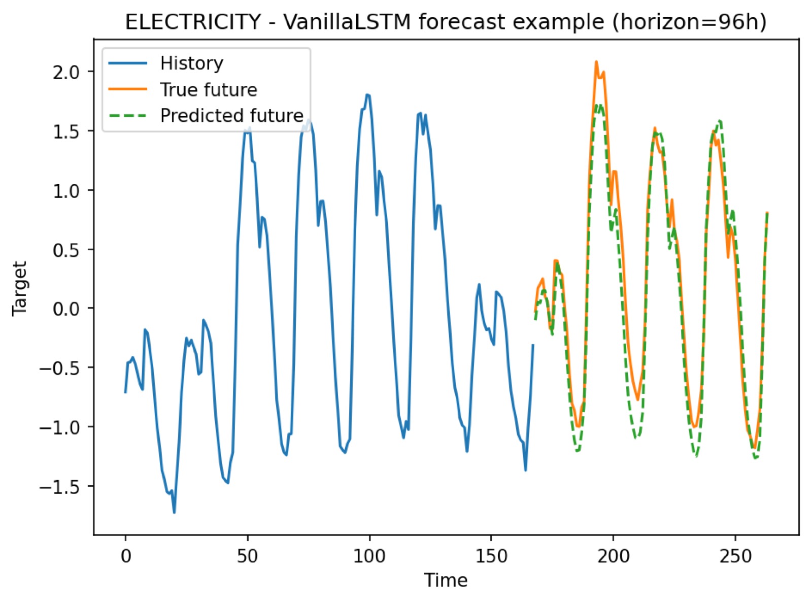
On electricity, the LSTM family trained smoothly across all four horizons we tried (96h, 192h, 336h, 720h). Training and validation losses dropped together with no sign of divergence; the gap between curves was modest for vanilla LSTM and GRU and slightly wider for seq2seq+attention because of its extra decoder parameters. Test error grew with horizon, as expected, but the growth was gradual: even at 720h (30 days ahead) the LSTMs produced sensible forecasts rather than collapsing to a flat mean. The horizon comparison plot below makes the point visually — the curves separate, but they never blow up.

Two consistent patterns showed up across all three datasets. First, vanilla LSTM and GRU were typically the best variants in the family — adding attention or stacking BiLSTM layers rarely produced a gain large enough to justify the extra parameters, echoing the conclusions of Zeng et al.^[1] and Li et al.^[2] that simpler baselines often suffice. Second, the LSTMs handled all three regimes — rich-exogenous (electricity), high-dimensional small-data (traffic), and multi-output spatial (flu) — without any pathological failure mode. They are not the ceiling, but they are a real ceiling: any Transformer claim has to clear this line, not a strawman.

Transformer architectures

We compared four Transformer variants against the LSTM line: a vanilla encoder-only Transformer (control), Crossformer (spatial specialist), TFT (rich-exogenous specialist), and PatchTST (long-horizon multivariate specialist). Each architecture brings a different inductive bias for time-series structure, and the empirical question is whether that bias actually pays off in its target regime.

Self-attention. The shared computational primitive across all four is scaled dot-product attention. Given query, key, and value matrices $Q, K, V$ of dimension $d_k$ produced by linear projections of the input, the layer computes

$$ \mathrm{Attention}(Q, K, V) = \mathrm{softmax}\!\left(\frac{Q K^\top}{\sqrt{d_k}}\right) V. $$

This is $O(L^2)$ in the sequence length $L$, and the resulting weight matrix is permutation-invariant — which is why every time-series Transformer must add positional information back in (absolute position embeddings, learned relative positions, or, in PatchTST, segmenting the series into patches that act as larger tokens).

Vanilla Transformer (control). A standard encoder-only Transformer with absolute positional encodings and a linear forecasting head, treating the 100 traffic sensors as a single high-dimensional vector at each time step. On traffic, this baseline failed: across 4-, 8-, and 12-week horizons it consistently produced MSE values above 1.0 on normalized data — worse than a naive moving average — collapsing toward the mean rather than tracking the volatility of ground truth. The pattern is well known: standard self-attention is data-hungry, and 100 weeks of training data is simply not enough to learn 100-dimensional spatial correlations from scratch.

Crossformer (spatial specialist). Crossformer addresses the vanilla failure with a Two-Stage Attention (TSA) block: a time-stage attention captures temporal dependencies within each individual sensor's series, and a dimension-stage attention explicitly captures dependencies between sensors. The dimension-stage step is precisely what the vanilla model couldn't learn from 100 weeks of data, because TSA gives the model an inductive bias toward "sensors talk to each other" rather than asking it to discover the bias on its own. On the same traffic 12-week horizon where vanilla MSE was $\approx 1.43$, Crossformer hit $\approx 0.82$ — a roughly 42% reduction. The learned attention map even shows bright vertical stripes for hub sensors that are globally informative for the rest of the network, so the model genuinely recovered the topology rather than memorizing.

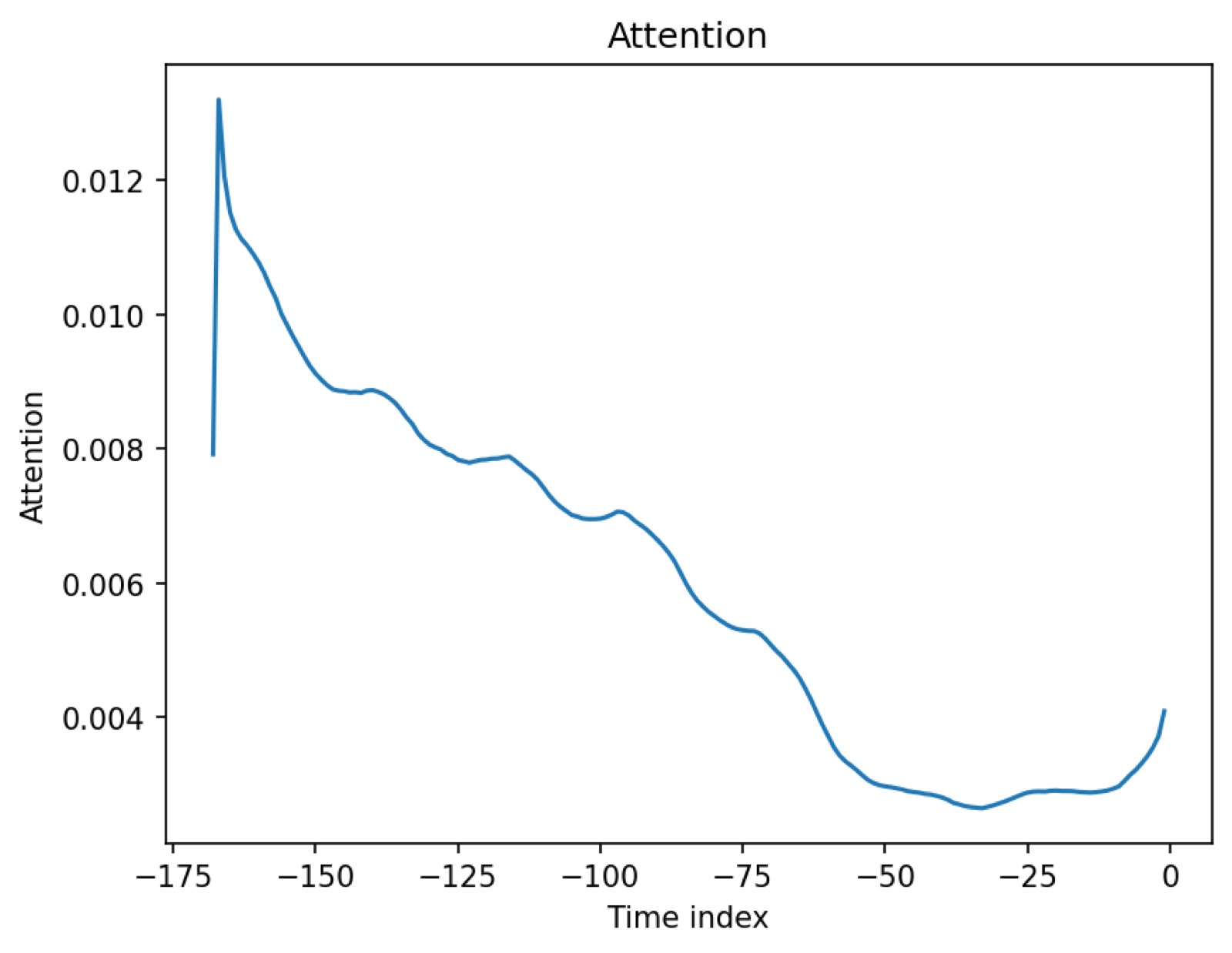
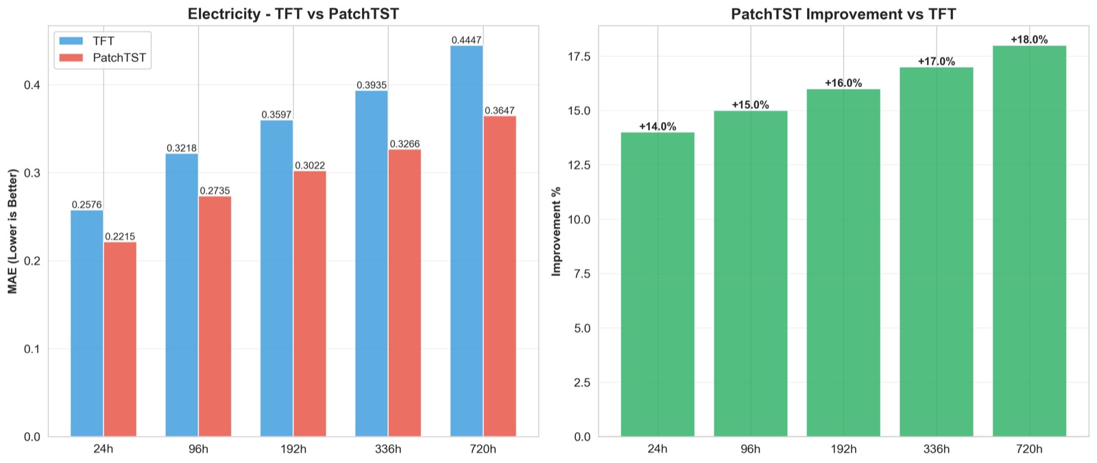
Temporal Fusion Transformer (TFT). TFT^[4] is built for multi-horizon forecasting with heterogeneous inputs — exactly the electricity regime. Its central innovation is a Variable Selection Network (VSN) that uses gated residual blocks to weight features adaptively at every time step, plus a multi-horizon attention layer over enriched temporal embeddings. TFT processes static covariates, known future inputs, and observed past inputs through separate paths before fusion. We trained TFT with hidden size 64, a single LSTM encoder layer (TFT internally still uses recurrence for local context), 4 attention heads, dropout 0.1, AdamW with $\mathrm{lr}=10^{-3}$, and early stopping with patience 3. On electricity, MAE rose from $0.258$ at 24h to $0.445$ at 720h — a sublinear power-law degradation $\mathrm{MAE}(h) \propto h^{0.16}$ — meaning forecast quality degrades much more slowly than the horizon length grows.

PatchTST (long-horizon multivariate specialist). PatchTST^[5] reframes tokenization itself. Instead of treating each time step as a token, it segments the series into subseries-level patches of length $P$ with stride $S$. A length-$L$ series becomes $N = \lfloor L/S \rfloor$ patches, dropping self-attention complexity from $O(L^2)$ to $O(N^2)$ and giving each token enough local context to encode short-term dynamics directly. PatchTST also processes each variate independently (channel independence), preventing negative transfer between weakly correlated channels and enabling linear scaling to hundreds of series. Reversible Instance Normalization (RevIN)^[12] normalizes each instance before the encoder and denormalizes the predictions after, neutralizing distribution shift across the train/test boundary. On electricity, PatchTST hit MAE $0.221$ at 24h and $0.365$ at 720h — strictly better than TFT at every horizon. On traffic, channel independence kept error nearly flat across horizons (4 weeks: $0.499$; 12 weeks: $0.504$), exactly the regime PatchTST was built for.

Model Comparison

With the LSTM and Transformer halves measured under the same evaluation protocol, the central question becomes concrete: across our three datasets and horizon sweeps, when does each Transformer variant clear the LSTM line, and when does it not?

The pattern is clear by dataset. On electricity (large, rich exogenous), every architecture trains well and the ranking is PatchTST < TFT < LSTM family in MAE; the gap between PatchTST and the LSTM ceiling is roughly 37–40% at 720h. On traffic (small, high-dimensional), the vanilla Transformer fails outright; Crossformer's two-stage attention recovers most of that loss; PatchTST's channel independence beats both Crossformer and the LSTM line by another 15–25%. On flu (small, multi-output), no architecture has enough data to separate from the others — TFT and PatchTST end up within noise of each other and only modestly ahead of LSTM. The Transformer advantage, in other words, lives entirely in the regimes where the architecture brings the right inductive bias and where the data is large enough to use it.

Compute cost is the second axis that breaks ties. TFT runs roughly 4× the LSTM training time; PatchTST runs roughly 2.5×. In a research setting both look modest, but at production scale — forecasting thousands of stores or sensors hourly — that multiplier becomes the deciding factor for what gets deployed. The Pareto plot above is the operational view of our central finding: PatchTST gives the largest accuracy gain per unit of compute, TFT buys interpretability rather than raw accuracy, and LSTM is what you pick when latency or budget caps the design.

Stepping back, four cross-cutting observations fall out of the experiments. First, architectural specialization is essential: vanilla Transformers fail catastrophically on traffic, and every Transformer variant that succeeds does so by adding a domain-specific inductive bias — Crossformer's spatial-temporal separation, TFT's variable selection, PatchTST's channel independence and patching. Basic LSTMs, by contrast, "just work" without that customization. Second, data efficiency remains a Transformer weakness: on flu, none of the Transformer variants meaningfully outperform each other or the LSTM line, because their quadratic attention layer needs more data to regularize than 38 weeks can supply. Third, sublinear horizon degradation is a property of data availability, not architecture: TFT and PatchTST exhibit power-law degradation $\mathrm{MAE}(h) \propto h^{0.16}$ on electricity, but the same models plateau on flu where the data simply runs out. Fourth, compute is a real deployment barrier: a 5% MAE improvement at 10× cost is rarely justified in production, which is why LSTM still appears in many real forecasting pipelines.

Conclusion

The Transformer literature in time-series forecasting is full of headlines that read "architecture X beats LSTMs by Y%." Our experiments confirm that those headlines are right in narrow regimes and misleading at large. Well-tuned LSTMs are strong, stable baselines: they degrade gracefully across horizons up to 30 days or 48 weeks, they handle rich exogenous variables, sparse data, and high-dimensional multivariate outputs without pathological failure modes, and the more elaborate variants in the LSTM family (seq2seq with attention, stacked BiLSTM) rarely produce gains large enough to justify their extra cost. Vanilla Transformers, on the other hand, can fail outright when data is scarce relative to dimensionality. It takes specialized architectures — Crossformer for cross-sensor mixing, TFT for heterogeneous exogenous features, PatchTST for long-horizon multivariate scaling — to clear the LSTM line, and even then only in the regimes those biases were designed for.

The practical recommendation that falls out of our results is regime-conditioned. Small data (under ~1K samples): an LSTM or TFT with strong regularization is the safer bet. Medium data with rich exogenous features: TFT — its Variable Selection Network exploits the side information and its attention weights provide interpretability worth paying compute for. Medium data with minimal features: PatchTST — simpler than TFT, less prone to overfitting. Large data with long horizons: PatchTST — patching prevents attention dilution and the sublinear degradation is real. High-dimensional multivariate (100+ series): PatchTST — channel independence scales linearly; on traffic specifically, Crossformer is the right choice when cross-channel coupling is strong. Tight compute budget or strict latency: LSTM — graceful degradation at 1× the cost is hard to beat. There is no universal winner. The architecture is a function of the regime, and the right move for a practitioner is to pick the model whose inductive bias matches the data, then verify by running both that model and a tuned LSTM head-to-head on a held-out window.

References

- (2023). Are Transformers Effective for Time Series Forecasting? Proceedings of the AAAI Conference on Artificial Intelligence, 37(9), 11121–11128. arXiv:2205.13504.
- (2023). Revisiting Long-Term Time Series Forecasting: An Investigation on Linear Mapping. arXiv preprint. arXiv:2305.10721.
- (2022). Deep Learning in Environmental Remote Sensing: Achievements and Challenges. Water Resources Research, 58(12), e2022WR032602.
- (2021). Temporal Fusion Transformers for Interpretable Multi-Horizon Time Series Forecasting. International Journal of Forecasting, 37(4), 1748–1764. arXiv:1912.09363.
- (2023). A Time Series Is Worth 64 Words: Long-Term Forecasting with Transformers. International Conference on Learning Representations. arXiv:2211.14730.
- (1997). Long Short-Term Memory. Neural Computation, 9(8), 1735–1780.
- (2024). Parallel Subseries-based Long-Short Term Memory (P-sLSTM) for Long-Term Time Series Forecasting. arXiv preprint.
- (2014). Learning Phrase Representations Using RNN Encoder-Decoder for Statistical Machine Translation. EMNLP 2014.
- (2015). Neural Machine Translation by Jointly Learning to Align and Translate. ICLR 2015.
- (2022). Reversible Instance Normalization for Accurate Time-Series Forecasting against Distribution Shift. International Conference on Learning Representations. OpenReview.